Suppose a cyclist is resting at some point in his hike at a point P located 20 km from a city 0. It resumes its route away from this city 0 at a speed of 15 km / h.
a) How far from town 0 will it be after 1 hour ? 2 hours ? 3 hours ? etc ...
b) What is the graph that can represent the distance traveled as a function of time ?
Solution:
a) We know that the distance traveled by a person or a moving object, called a "mobile", is a function of the speed of this mobile and its travel time.
The distance traveled by the cyclist in one hour is 15 x 1 = 15 km. It is therefore distant from the city 0 of 15 + 20 = 35 km (point P1 Figure 7).
In two hours, he travels : 15 x 2 = 30 km. It is then 30 + 20 = 50 km from 0 (point P2).
Generalize: in x hours, the cyclist travels 15. x km. It is then found at 15 x + 20 km of 0.
Let y denote the cycling distance - city 0. The relation linking this distance (y) to the travel time (x) can therefore be written :
y = 15x + 20
If we replace the numbers 15 and 20 by the letters a and b, called parameters, that is to say letters representing any but known numbers, the relation becomes :
y = ax + b
b) Graph the function y = 15 x + 20. Let's take a scale of 1 cm = 10 km and 1 cm = 1 hour.
Let us determine the points P1, P2, P3, etc., whose respective coordinates are the corresponding values of x and y (Figure 7).
Point P x = 0
y = (15 X 0) + 20 = 20
Point P1 x = 1
y = (15 X 1) + 20 = 35
Point P2 x = 2
y = (15 X 2) + 20 = 50
Point P3 x = 3
y = (15 X 3) + 20 = 65
etc....
By joining the points to each other, we see that they are aligned and that consequently the curve representative of the function y = 15x + 20 is a straight line.
5. 2. - REPRESENTATION OF THE FUNCTION y = ax + b
By generalizing what has just been said, we can write :
The representative curve of the function y = ax + b is a line parallel to the line y = ax and intersecting the ordinate axis at the ordinate point b.
Remarks and definitions:
The number b is called the ordinate at the origin (value of y for x = 0),
The line y = ax + b being parallel to the line y = ax has the same slope ; the parameter "a" is the slope (or angular coefficient) of the line y = ax + b.
If "a" is positive, the function y = ax is increasing. The two lines being parallel, the function y = ax + b is also increasing.
The parameter "b" can be positive or negative. If it is zero, the equation reduces to y = ax.
For the same reason, if "a" is negative, the function y = ax and consequently the function y = ax + b are decreasing.
In summary, in the function y = ax + b :
a is the slope ;
b is the order of origin, positive or negative ;
si a > 0 the function is increasing ;
si a < 0 the function is decreasing.
5. 3. - PRACTICAL PRACTICE OF THE RIGHT y = ax + b
To construct the line y = ax + b, it suffices, of course, to determine two of its points and to join them. In general, we determine the points that result from the intersection of this line with the coordinate axes :
we make x = 0 and we calculate y ;
then y = 0 and we calculate x.
First example : Let the function
y = - 2x + 4
Take as scale :
for the x-axis 2 cm = one unit
for the y-axis 1 cm = one unit
Let's draw the two axes (Figure 8)
Let x = 0;
the relation y = - 2x + 4 becomes :
y = 0 + 4 = 4 (points P1)
Let y = 0;
the relation y = - 2x + 4 becomes :
0 = - 2x + 4
from where
2 x = 4
is
x = 2 (point P2)
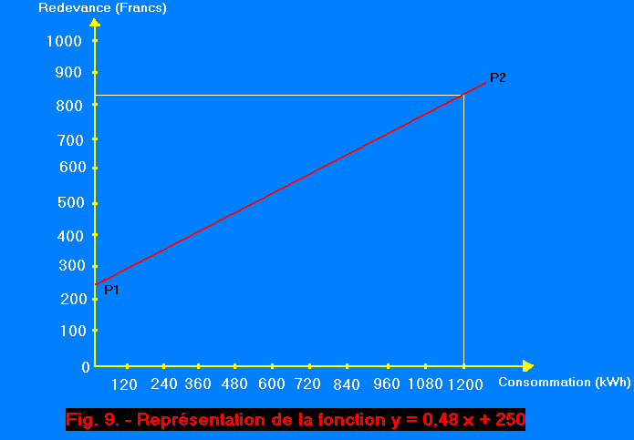
Price payable = number of kWh consumed X price per kWh
What is of the form : y = ax by attributing "y" to the price to be paid, "x" to the number of kWh consumed and "a", known parameter, at the price of kWh that is to say 48 cents..
It remains to take into account the rental of the meter which is fixed and independent of consumption. Here we have the factor b and we can write : y = ax + b.
With y = amount of the fee
a = price per kWh (0,48 F)
x = number of kWh consumed
b = rental of the meter (250 Francs)
and numerically : y = 0.48x + 250
The relationship being established, we need to transpose graphically.
To draw and scale the coordinate axes, choose the scales :
- Horizontal axis. We have a maximum consumption of 1200 kWh. Taking an axis of 10 cm, we get 1200 / 10 = 120 kWh per centimeter.
- Y axis. At the maximum, the fee will be :
(0,48 X 1 200) + 250 = 576 + 250 = 826 francs.
With an axis of 10 cm, we obtain 826 / 10 = 82.6 F per centimeter. For convenience, we will take 100 F per centimeter.
Let's draw and scale the two axes (Figure 9).
Let's determine the two points needed to draw the line.
We have y = 0,48 x + 250
For x = 0 y = 250 (P1)
For y = 0 0 = 0,48 x + 250 - 0,48 x = 250
x = - 250 / 0,48 = - 520
We do not have this value on our chart. We could find it by extending the x-axis to the negative values. But let's do otherwise. Suppose our consumption is 1 200 kWh which corresponds to a fee of :
y = 0,48 . 1 200 + 250
y = 826
We have thus determined the coordinates of the second point : P2 (1 200 , 826). The two points being found, it remains only to draw the line.
In electrotechnics or electronics, we find laws whose general form is y = ax + b.
In the study of transistors, we find the relation :
Definition :
A quantity is proportional to the square of another when one having a value, the other takes the square of this value.
Consider a resistance in which a current I of different values is passed. A wattmeter connected in the circuit allows us to measure the power P consumed by this resistance :
I
1
2
3
4
5
P
10
40
90
160
250
Now let us establish the ratios between the powers and the square of the corresponding currents.
We notice that this report is constant. The value obtained in our example (10) is that of the resistance R.
We can write :
R = P / I2
In general, if (x) is the measure of a magnitude and (y) the measure of another magnitude proportional to the square of the first, the ratio of proportionality "a" is expressed by the relation :
a = y / x2 or y = ax2
The definition of the beginning of the paragraph can thus be expressed as follows : a quantity (y) is proportional to the square of a quantity (x) when they are linked by the relation : y = ax2, "a" being a fixed coefficient.
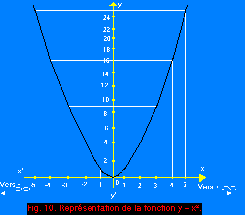
In the case where a = 1, the function y = ax2 is reduced to y = x2.
To graphically study the function y = x2, we will give x any positive and negative values. Each of these values, squared, will give the corresponding value of y.
Let's write the sequence of integers and their squares below :
x =
- 5
- 4
- 3
- 2
- 1
0
1
2
3
4
5
y = x2 =
25
16
9
4
1
0
1
4
9
16
25
In examining this table we notice :
When the negative numbers increase, that is to say when they get closer to zero, their squares decrease,
When positive numbers increase, their squares increase,
Two opposite numbers have the same square.
The results obtained are graphically represented in Figure 10 (the method for drawing a curve is now assumed to be known, we will no longer explain it in detail).
We note that the curve obtained is no longer a straight line as in the case of two directly proportional quantities. This curve is called a parable.
On the other hand, we can observe that :
- The function is defined for all values of x ; in other words, whatever x (x may vary from
- +),
we can always calculate its square x2;
- The function is always positive, except for x = 0, value for which y = 0
- When x is given two opposite values, y has the same value : If x is equal to - 3 or + 3, y = 9 in both cases. In other words, the curve admits the axis y'y as axis of symmetry ;
- When x varies from -
to 0, the function is decreasing ; when x varies from 0 to + ,
it is increasing ;
- The function goes through a minimum x = 0 ;
- When x increases indefinitely by positive or negative values, it increases indefinitely.
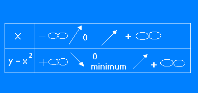
The study of the variation of the function y = x2 can be summarized by the following table which we will use again later.
In the first line of this table, we find different values of x. Here we have taken the extreme values -and +and the value zero. In the study of functions a little more complicated, we take other particular values as we will see. The inclination of the arrows gives the direction of variation of the numbers lying between the two values located on either side of the arrow when one counts the value located on the left of this one to arrive at that which is located at right. Thus, when one starts from-
to arrive at zero, the relative values of the numbers increase as one approaches 0 ; we summarize this by an arrow to which we give an ascending inclination. When we start from 0 and continue counting indefinitely, the values of the numbers also increase and the arrow is still ascending.
The second line gives the values of the function calculated from those of the variable in the first row. When starting from +to zero, it is obvious that the values of numbers are smaller and smaller, hence the downward arrow.
On the contrary and as before, when we count from zero to infinity, the values increase and the arrow is ascending.
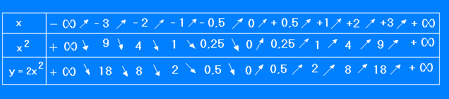
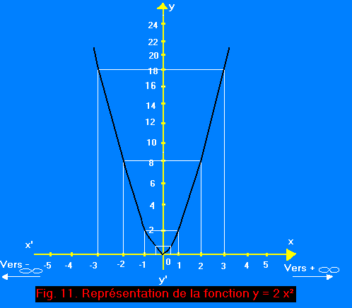
7. 2. - FUNCTION y = 2 x2
This function can be in the form :
y = x2 X 2
So, to calculate y, it is enough to multiply by 2 the values obtained for x2.
Let's do these calculations for some arbitrary values of x, write the results in the following table and symbolize with arrows, as we have seen, the meaning of the variations.
By analyzing the table, we see that for the values of :
- x varying from -to 0:y decreases from +to 0
- x varying from 0 to +
:y increases from 0 to +
The curve of Figure 11 materializes the different results.
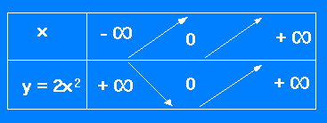
Note :
The tables and charts do not always show the calculations and intermediate values used to construct the curve. The table is simplified and then looks like this :
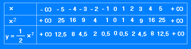
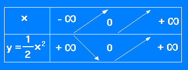
7. 3. -FUNCTION y = (1
/ 2) x2
As before, let us start with the table of the study of the variations of (y) according to those of x.
The summary table is as follows :
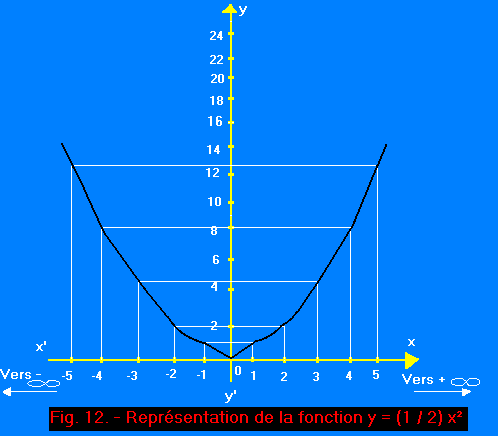
Now let's draw the corresponding curve (Figure 12).
We see that the curve obtained is always a parable.


 Proportional size squared of another size
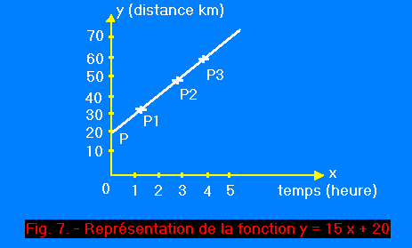
 Click here for the next lesson or in the summary provided for this purpose
 Top of page
 Next Page