 Comparison with Karnaugh's method Comparison with Karnaugh's method |
 Synthesis Synthesis
|
 Karnaugh's Table Karnaugh's Table
|
 Simplification of functions Simplification of functions
|
 Footer Footer |
Quine-Mac Cluskey Method and Comparison with the Karnaugh Method :
4. - QUINE-MAC CLUSKEY METHOD
Although little used, we still have to use a different method than Karnaugh's tables for simplifying the functions of several variables. It is a method devised by the American mathematician W. V. QUINE and remodeled by his fellow Dr. Edwards J. Mac CLUSKEY Junior in a doctoral thesis he presented to the M. I. T. (Massachusetts Institute of Technology) in June 1956.
4. 1. - DESCRIPTION OF THE METHOD
To examine this method, we will take an example with four variables. Let us start from the truth table of the function f (a, b, c, d) which is given in Figure 54.
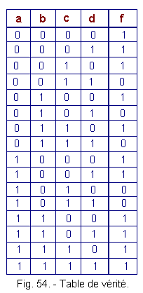
We can see that the function f is "true" (equal to 1) for eleven combinations of the variables a, b, c and d.
Give each of these combinations a name for the decimal value, which corresponds to the binary code formed by the variables a, b, c, d, considering that a is the most significant bit and d is the least significant bit.
Example :
0110 = ![]() bc
bc![]() : we will call it the combination 6 since 0110 in binary equals 6 in decimal.
: we will call it the combination 6 since 0110 in binary equals 6 in decimal.
If we recapitulate, then the function f is the sum of the combinations summarized in figure 55 :
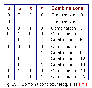
This list can be summarized as follows :

From this list of combinations actually begins the QUINE-MAC CLUSKEY method.
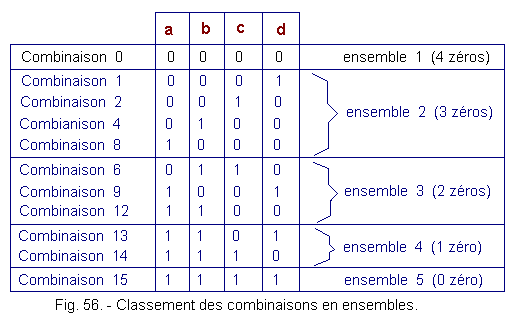
The first thing to do is to classify these combinations into a successive set according to the number of zeros in the binary form of each combination, starting with the one that counts the most.
The first set is formed by the combination 0 whose binary form 0000 has four zeros. The second set includes combinations with three zeros ... up to the fifth which is formed of the combination 15 whose binary form 1111 does not have zero at all.
The five sets are shown in Figure 56.
The second phase of the method consists in comparing the terms of each set with the terms of the set immediately following so as to eliminate a variable if it is possible.
The combination 0000 of the set 1 must therefore be compared to the four combinations of the set 2. Then each of the four combinations of this set 2 will be compared to each of the three combinations of the set 3 and so on until set 5 ...
When two combinations differ only from ONE VARIABLE, they can be combined to form only one in which the variable that differs can be eliminated.
When a variable is eliminated in such an association, this fact is indicated by replacing this variable with a cross (or any other sign at your convenience).
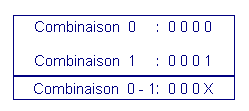
In the example we have chosen, the combinations 0 and 1 can, for example, be associated since only the variable d is different :
Let us proceed thus by comparing each term of each set with each term of the following set and we obtain the combinations described in Figure 57.
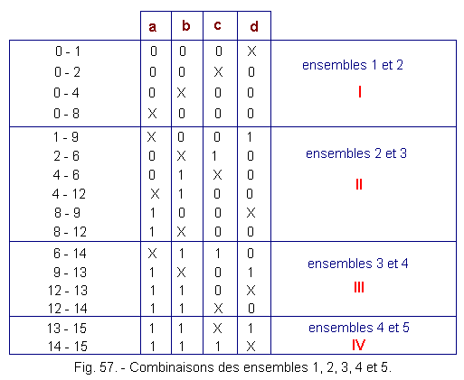
We are getting new members now grouped into four sets I, II, III and IV. Let's do the same thing again with these new sets. Figure 58 gives the new combinations obtained.
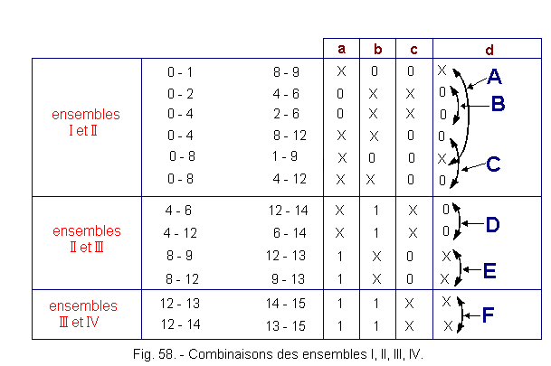
In the general principles of the QUINE-MAC CLUSKEY method, it is advisable to continue this process until there is no longer any possible combination between one of these sets and the next.
In the example chosen, we arrived at this point. Moreover, we note in this figure that several combinations are identical. We will of course keep only the different groupings we will call A, B, C, D, E and F (Figure 58).
The function f then takes the form :
f = A + B + C + D + E + F, Let :
f = ![]()
![]() +
+ ![]()
![]() +
+ ![]()
![]() + b
+ b![]() + a
+ a![]() + ab
+ ab
NOTE :
In all the groupings that we have made, it could have happened that some terms of a set do not combine with any term of the following set. These terms are then prime terms and should not be forgotten in the final equation.
At this point, it must be verified whether the equation obtained can not yet be simplified. To eliminate any superfluous terms, let us form a grid called "diagram of the first terms".
This diagram shown in Figure 59 comprises eleven columns corresponding to the initial combinations 0, 1, 2, 4, 6, 8, 9, 12, 13, 14 and 15. It also comprises six horizontal lines corresponding to the six groups A, B , C, D, E and F obtained after the various simplification processes.
On each line, mark with a cross the combinations that served to form the group considered.
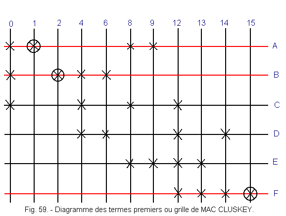
For example for the group A which involves the combinations 0, 1, 8 and 9, we checked on line A the columns 0, 1, 8 and 9. After doing the same for the lines B, C, D, E and F, we find that some columns (1, 2 and 15) have only one cross that we then surround a circle. These combinations are located on the lines A, B, and F which are called "baselines".
We note that on the other hand the combinations included in the lines C, D, E are found at least once in the lines A, B and F. The lines C, D and E can be removed and the function f is simplified. so again to become :
f = A + B + F
f = ![]()
![]() +
+ ![]()
![]() + ab
+ ab
![]() 4. 2. - COMPARISON WITH KARNAUGH'S METHOD
4. 2. - COMPARISON WITH KARNAUGH'S METHOD
For comparison, let's do the same exercise using the KARNAUGH tables method. Using the truth table recalled in Figure 60-a, let us draw up the corresponding KARNAUGH table (Figure 60-b).
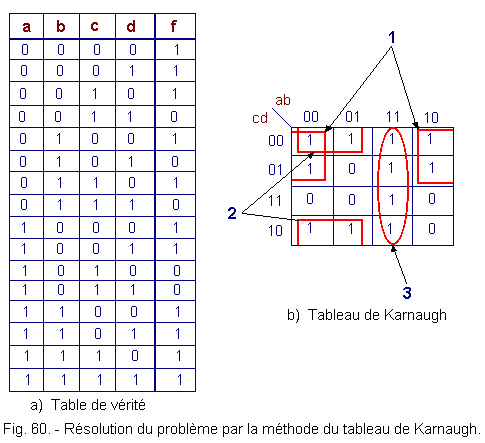
The groupings made in this table (circled in red in the figure) immediately give the solution :
f = 1 + 2 + 3
f = ![]()
![]() +
+ ![]()
![]() + ab
+ ab
We find the same result as before.
CONCLUSIONS :
In the light of this example, solved on the one hand with the method of QUINE MAC CLUSKEY, on the other hand thanks to a painting by Karnaugh, it appears that the second is much simpler, faster and more seductive than the first. This explains why this first method is almost unused. We will not dwell on it anymore.
It should be noted, however, that this method of QUINE MAC CLUSKEY applies regardless of the number of variables, whereas the method of Karnaugh's tables becomes significantly more complicated when the number of variables increases and becomes greater than 6 or 7.
![]() 5. - SYNTHESIS
5. - SYNTHESIS
In this chapter called synthesis, we will make a reminder of all the important notions necessary for the study and the realization of circuits and diagrams of combinational logic electronics since the combinatorial logic was the object of our concern in the three first theories.
Indeed, we call combinatorial logic any circuit in which the outputs are only a function of the values of the inputs, regardless of time.
5. 1. - VARIABLE
A logical variable is any quantity that can take only two values, 1 or 0.
5. 2. - FUNCTION
When two simple Boolean variables a and b vary in such a way that for each value of a corresponds a well-defined value of b, the quantity b is a function of a.
We write b = f (a).
5. 3. - TABLES OF TRUTH
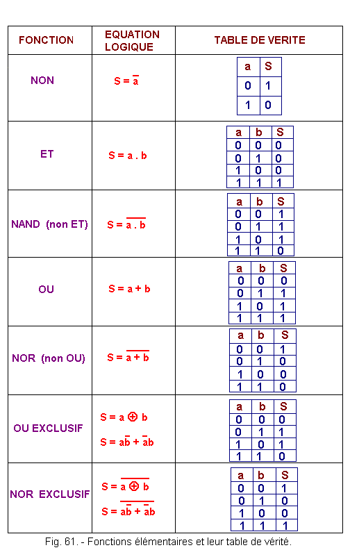
Figure 61 summarizes the various basic logic functions.
For each logical function, there corresponds a truth table and a logical equation. The truth table indicates the state of the output of the function considered, according to the state of the input variables.
5. 4. - GRAPHIC SYMBOLS
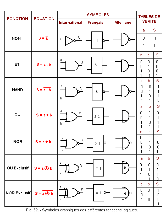
Figure 62 gives the different graphical representations used for the logic functions.
![]() 5. 5. - KARNAUGH TABLES
5. 5. - KARNAUGH TABLES
![]() The number of boxes, constituting the array, is a function of the number of variables involved. We saw that a variable could take two states : "1" or "0".
The number of boxes, constituting the array, is a function of the number of variables involved. We saw that a variable could take two states : "1" or "0".
![]() Two variables can take four combinations of states :
Two variables can take four combinations of states :
1 Þ "0" and "0"
2 Þ "0" and "1"
3 Þ "1" and "0"
4 Þ "1" and "1"
![]() The number of possible combinations is given by the formula :
The number of possible combinations is given by the formula :
x = 2n with n = numbers of variables.
5. 5. 1. - TABLE OF KARNAUGH HAS ONLY ONE VARIABLE
Example : fonction YES, x = a.
![]() The electrical state of S
is only a function of "a". we have :
x = 21 = 2 boxes.
The electrical state of S
is only a function of "a". we have :
x = 21 = 2 boxes.
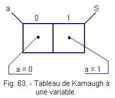
Figure 63 gives Karnaugh's table of this function.
5. 5. 2. - TABLE OF KARNAUGH HAS TWO VARIABLES
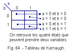
Figure 64 gives the configuration of the Karnaugh table in the case of two variables.
Example : S = a + b x = 22 = 4 cases
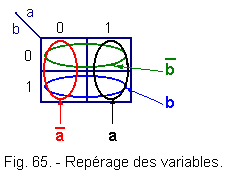
a) Locating the two variables :
![]() The state "1" of a variable occupies half of the boxes,
The state "1" of a variable occupies half of the boxes,
![]() The state "0" one variable occupies the other half (Figure 65).
The state "0" one variable occupies the other half (Figure 65).
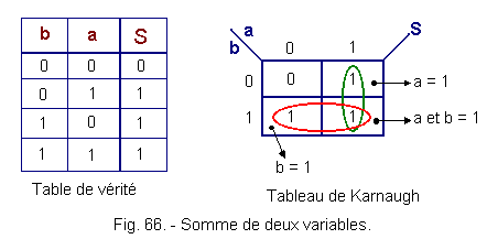
b) Locating a sum of two variables :
![]() This sum is represented by all the boxes belonging to the two variables,
This sum is represented by all the boxes belonging to the two variables,
![]() The identification will be done by "0" and "1" which have the same meaning as in the truth tables, see S = a + b.
The identification will be done by "0" and "1" which have the same meaning as in the truth tables, see S = a + b.
Figure 66 gives the truth table and the corresponding Karnaugh table.
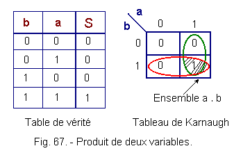
c) Locating a product of two variables :
![]() This product is represented by the set of boxes common to both variables as for Euler circles, Let
S = a . b.
This product is represented by the set of boxes common to both variables as for Euler circles, Let
S = a . b.
Figure 67 gives the truth table and the corresponding Karnaugh table.
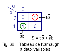
d) Locating any two-variable function :
See S = a![]() +
+ ![]() b,
Figure 68 gives the corresponding Karnaugh table.
b,
Figure 68 gives the corresponding Karnaugh table.
We first identify the product
a![]() then the product
then the product ![]() b.
b.
5. 5. 3. - TABLE OF KARNAUGH HAS THREE VARIABLES
x = 23 = 8 cases
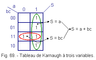
See S = a + bc, Figure 69 gives Karnaugh's table of this function.
5. 5. 4. - TABLE OF KARNAUGH AT FOUR VARIABLES
x = 24 = 16 cases
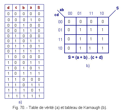
See S = (a + b) . (c + d), The truth table and Karnaugh's table of this function are shown in Figure 70.
5. 5. 5. - CASE OF MORE THAN FOUR VARIABLES
We use several Karnaugh tables with four variables that are superimposed. Their number doubles each time we add a new variable beyond four.
Example : 4 variables = 1 board
5 variables = 2 paintings
6 variables = 4 paintings
7 variables = 8 paintings
One can also use the method of Mac CLUSKEY seen previously.
![]() 5. 6. - SIMPLIFICATION OF FUNCTIONS
5. 6. - SIMPLIFICATION OF FUNCTIONS
The representation of the functions on a Karnaugh board makes it possible to quickly detect simplifications.
5. 6. 1. - RULE :
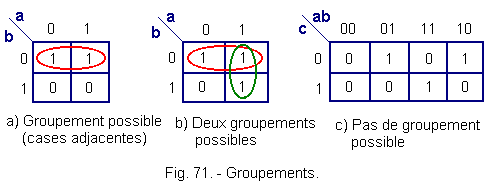
![]() The minimal equation will be obtained by practicing the maximal groupings by power of (2, 4, 8 cases), of adjacent squares.
The minimal equation will be obtained by practicing the maximal groupings by power of (2, 4, 8 cases), of adjacent squares.
![]() The expression of a group contains only those variables that do not change state (Figure 71).
The expression of a group contains only those variables that do not change state (Figure 71).
![]() Another type of grouping possible :
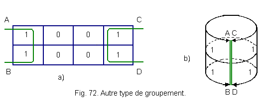
Another type of grouping possible :
The table in Figure 72 should be considered as rolling over itself to meet on the AB and CD lines or on the AC and BD lines.
Only the surface of a torus could make this image (Figure 72-b).
When the groupings are realized, we deduce the minimal equations.
5. 6. 2. - EXAMPLES :
![]() Either the function S = a + ab whose Figure 73 gives the table of Karnaugh
Either the function S = a + ab whose Figure 73 gives the table of Karnaugh
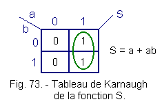
The equation deduced from the grouping is S = a, a is the only variable that in this group does not change state.
![]() Simplify the function : L =
Simplify the function : L = ![]()
![]() + a
+ a![]() +
+ ![]() b
b
Figure 74 gives the corresponding Karnaugh tables..
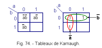
The simplified equation is :
L = ![]() +
+ ![]()
![]() Simplify the function : L = bd +
Simplify the function : L = bd + ![]()
![]()
![]() + a
+ a![]() cd
+
cd
+ ![]() c
c![]() + abc
+ abc![]()
Figure 75 gives the corresponding Karnaugh tables.
.gif)
Hence the simplified equation :
L = ac + bd + ![]()
![]()
5. 7. - MORGAN THEOREM
1st theorem :
The sum complement is equal to the product of each of its complemented terms.
Thus, the complement of a + b is ![]() .
. ![]() .
.
We write : ![]() =
= ![]() .
. ![]() .
.
2nd theorem :
The complement of a product is equal to the sum of each of its complemented terms. Thus, the complement of a . b is ![]() +
+ ![]() .
.
We write : ![]() =
= ![]() +
+ ![]()
In the next chapter, we propose two solved problems that will allow you to put into practice all the knowledge acquired.
 Click here for the next lesson or in the summary provided for this purpose. Click here for the next lesson or in the summary provided for this purpose. |
|
 Previous Page Previous Page |
 Next Page Next Page |
Nombre de pages vues, à partir de cette date : le 27 Décembre 2019
Envoyez un courrier électronique à Administrateur Web Société pour toute question ou remarque concernant ce site Web.
Version du site : 10. 4. 12 - Site optimisation 1280 x 1024 pixels - Faculté de Nanterre - Dernière modification : 02 Septembre 2016.
Ce site Web a été Créé le, 14 Mars 1999 et ayant Rénové, en Septembre 2016.
