6. - FIFTH EXPERIENCE : REALIZING A DIGITAL THERMOMETER
The previous experiment showed you how to convert an analog voltage into a corresponding digital value.
However, this type of converter can not convert other physical quantities such as pressure or temperature.
To make a temperature measurement, it is therefore necessary, firstly, to convert the temperature into tenson and then, in a second step, to convert this voltage into a numerical value. The block diagram of Figure 25 represents these two conversion steps.
The conversion of the temperature into analog voltage is done through a transducer.
On the market, there are many types of temperature transducers. For example, thermistors whose resistive value is a function of temperature, thermocouples generating a voltage proportional to the temperature.
Temperature transducers, also known as temperature sensors, are distinguished by the range of temperatures at which they can work and also by the rate of reaction to temperature changes.
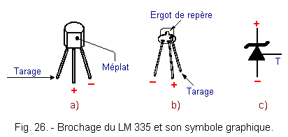
In this experiment, you will use the LM 335 integrated circuit.
As shown in Figure 26-a and 26-b, it is encapsulated in the same types of packages as the transistors.
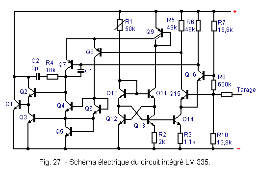
This circuit, shown in Figure 27, is quite complex and comprises sixteen transistors.
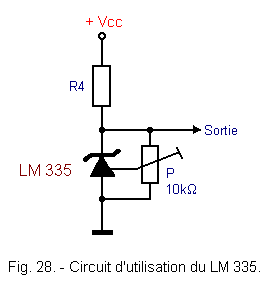
By cons, the use circuit shown in Figure 28 is relatively simple.
The voltage between the (+) and (-) terminals of the LM 335 is a function of the temperature.
At 25°C and with a current of 1 mA flowing in the sensor (LM 335), the typical value of the voltage is 2.98 volts. The minimum value is 2.92 volts and the maximum value is 3.04 volts.
The value of the resistor R4 must be calculated according to + Vcc so that the sensor is traversed by a current of 1 mA.
We take R4
= 2,2 kW which is a standardized value close to that calculated.
The output voltage is proportional to the temperature. It increases by 10 mV per additional degree Celsius.
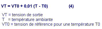
The relationship between voltage and temperature is given by the following formula :
VT is the output voltage, T is the ambient temperature, VT0 is the reference voltage for a temperature T0.
For T0 =
25° C and VT0 =
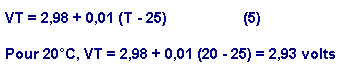
2,98 volts, we obtain :
To improve the accuracy of the measurement, the sensor calibration can be performed using a precision thermometer. With the latter, the temperature is measured and the value found in formula (5) is reported, which makes it possible to calculate VT.
All that remains is to adjust the output voltage to the calculated value. For this, use a precision voltmeter and act on the potentiometer P of 10 kΩ.
The sensor can work from - 10° C to + 100° C. For larger temperature ranges, there is the LM 135 (from - 55° C to + 150° C) and the LM 235 (- 40° C at + 125° C).
6. 1. - FIRST PART OF THE EXPERIENCE
6. 1. 1. - REALIZATION OF THE CIRCUIT
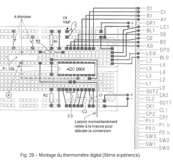
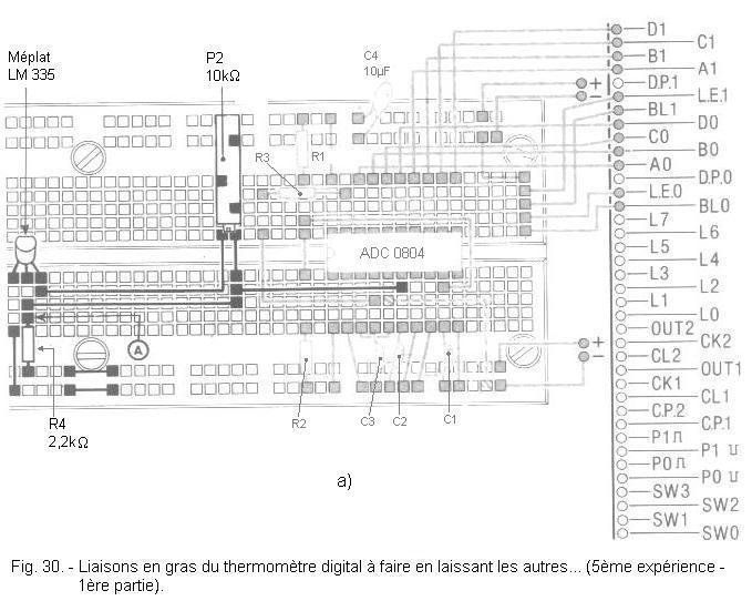
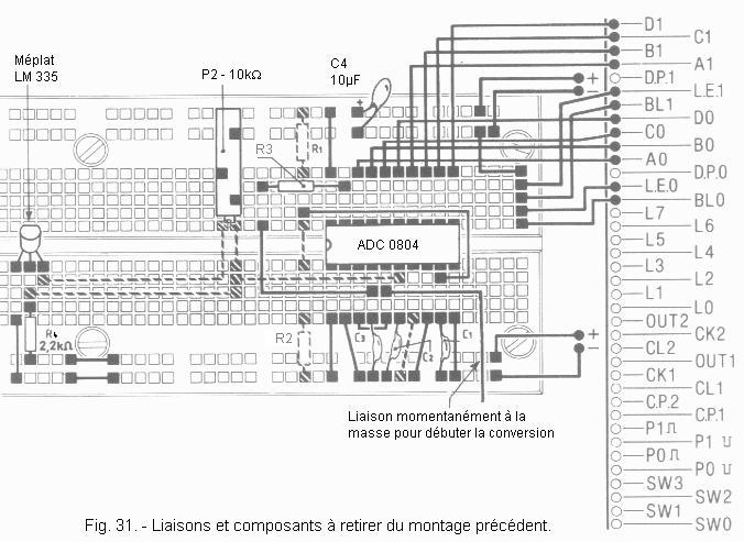
a) While retaining most of the previous assembly, remove the 10 kΩ potentiometer and the links shown in dotted line Figure 29.
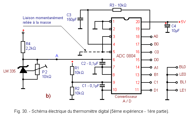
b) Insert the LM 335 circuit, the 2.2 kΩ R4 resistor and the 10 kΩ P2 potentiometer on the matrix as shown in Figure 30-a. Make the links highlighted in this figure.
The electrical diagram of the realized circuit is given in Figure 30-b.
6. 1. 2. - OPERATING TEST
a) Measure the room temperature with a thermometer to perform the circuit calibration.
b) Calculate the voltage VT using formula (5).
For example, for T
= 21° C, VT = 2,98 + 0,01 (21 - 25) = 2,94 volts
Now you need
to convert 2.94 volts to a hexadecimal value. To do this, use the tables in Figure 20 and Figure 21.
We must start with the most significant figure. In the table of Figure 21, the number immediately below 2.94 is 2.8125 which corresponds to the hexadecimal digit 9 on the DIS1 display.
The difference between
2,94 volts and 2,8125 volts is
0,1275 volt. In the table in Figure 20, it is 0,117 which is closest to 0,1275. The hexadecimal digit is 6.
Finally, at 21° C, the voltage across the sensor is 2.94 volts and the displays read 96.
c) Turn on the digilab.
d) Momentarily turn converter pin 5 to ground.
In all likelihood, the displays will not show the number you have calculated. In this case, perform the sensor calibration with the potentiometer P2 to display the correct hexadecimal number.
The LM 335 circuit is slow enough to follow temperature changes, its response time is about 5 minutes.
e) To take a measurement, raise the temperature of the LM 335 by squeezing it between your fingers.
f) Observe the displays, the number displayed increases slowly and stabilizes after a few minutes.
It is possible to calculate approximately the indication of the displays.
It can be assumed that the housing temperature of the LM 335 is approximately 32° C.
In this case, the voltage across the LM 335 is :
V32
= 2,98 + 0,01 (32 - 25) = 3,05 volts
Using the two tables previously used, we find the number 9 which corresponds to 2.8125 volts.
The difference 3.05 - 2.8125 = 0.2375 volts corresponds to the hexadecimal digit C.
The displays should indicate 9 C in this case.
g) The first part of the experiment is finished. Turn off the digilab.
This experience is particularly interesting because it presents a concrete use of an analog / digital converter.
Temperature measurement is of particular importance in some industrial control systems.
The proposed assembly is only didactic and does not lend itself to a practical application since the display does not indicate the temperature directly in ° C.
In real digital thermometers, the reading is done directly in ° C. For this, we use analog / digital converters that provide information in BCD code.
The mounting accuracy is not very high because the ADC 0804 converter has a resolution of 19.5 mV, while the voltage of the LM 335 varies by 10 mV per ° C.
In addition, the LM 335 has an accuracy of one degree and the converter an accuracy of ± 1 LSB.
All these errors are added and a relatively low accuracy of the digital thermometer results. However, if one limits the temperature range of the LM 335 circuit and changes the voltage range in which the converter operates, it becomes possible to directly display the temperature.
This is what we will do in the second part of the experiment.
6. 2. - SECOND PART OF THE EXPERIENCE
6. 2. 1. - REALIZATION OF THE CIRCUIT
a) While retaining most of the previous assembly, remove the resistors R1 and R2 and the six links shown in dotted line Figure 31.
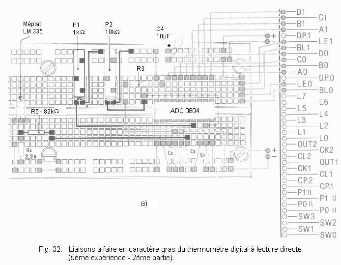
b) Insert on the matrix the potentiometer P1 of 1 kΩ and the resistance R5 of 82 kΩ as indicated Figure 32-a.
Make the indicated links highlighted in this figure.
The electric diagram realized is given in Figure 32-b.
Compared with the previous assembly, this makes it possible to vary the voltage range in which the converter operates. For this, there are two potentiometers P1 and P2.
The cursor of P1 connected to VIN (-) makes it possible to adjust the zero. For a temperature of 0° C, the displays will indicate 0 0.
The cursor of P2 connected to VREF / 2 makes it possible to adjust the scale factor of the converter, see the width of an LSB expressed in mV.
Thus, for a variation of 1° C, the hexadecimal display varies by one unit.
Consider the two temperatures 0° C and 100° C. The two voltages across the sensor are respectively worth :
V (0° C) = 2,98 + 0,01 (0 - 25) = 2,73 volts
V (100° C) = 2,98 + 0,01 (100 - 25) = 3,73 volts
In order for the displays to indicate 0 0 at 0° C, a voltage equal to 2.73 volts must be applied to the VIN (-) input with the potentiometer P1.
Furthermore, it is desired that at each temperature rise of 1° C, the indication of the displays increases by one unit. However, the voltage delivered by the sensor increases by an additional 10 mV per ° C. It is therefore necessary that the LSB corresponds to 10 mV. Since the transfer characteristic has 256 steps, the voltage scale must correspond to 10 mV x 256 = 2.56 volts.
Therefore, a voltage of 2.56 / 2 = 1.28 volts should be applied to the VREF / 2 input with the P2 potentiometer.
6. 2. 2. - OPERATING TEST
a) Place the controller on the 3 V gauge and place the test probes between pin 7 of the ADC 0804 circuit (red touch tip) and ground (black touch tip).
b) Set potentiometer P1 to read on the 2,73 volt galvanometer.
c) Similarly, set potentiometer P2 so that pin 9 of the ADC 0804 circuit is 1.28 volt.
With these two settings, the thermometer should be theoretically calibrated. In practice, it is not so.
Indeed, the two calculated voltage values are theoretical.
On the other hand, there are tolerances on the characteristics of the sensor and on the converter that can not be neglected.
Finally, the accuracy of the controller is also involved.
This is why a second calibration is interesting to increase the accuracy of the digital thermometer.
For this, you will use two reference temperatures : 0° C and the ambient temperature.
d) Put a few ice cubes in a perfectly sealed plastic bag or use aluminum foil.
e) Put the bag or foil containing the ice in direct contact with the sensor. Make sure that no drop of water falls on the digilab. If this happens, dry the matrix with a hair dryer.
The indication of the displays decreases. Wait a few minutes until it stabilizes. At this time, adjust potentiometer P1 so that display indication tends to change from 0 0 to 0 1.
f) Move the ice pack away, the display indication slowly increases. Wait several more minutes, then set the potentiometer P2 so that the indication of the displays is the same as that given by the thermometer (room temperature).
Remember that the indication of the displays is in hexadecimal code.
For 21° C, you must read 15 on the displays.
Indeed, 1516
= 2110
g) Repeat the two calibration operations described in phases e) and f) to increase the accuracy of the digital thermometer.
NOTE :
To achieve better accuracy in calibration, the set temperature range should be increased. For example, it should be set at 0° C and 100° C instead of 0° C and 21° C.
Moreover, the sensor may be at a temperature of 2 to 3° C higher than the ambient temperature since it is located above the digilab feed.
Now the thermometer is calibrated, you can make temperature measurements.
For this, you can cool the sensor with a fan or warm it with a lamp.
h) When the experiment is complete, turn off the digilab.
7. - GENERAL CONCLUSIONS
This last experiment allowed you to note that it was possible to better exploit the circuit ADC 0804, by modifying the range of the voltages for which it functions.
To do this, just apply half of this voltage range to the VREF / 2 input.
In addition, it is possible to "wedge" this voltage range between the extreme values 0 volt and 5 volts thanks to the input VIN (-).
In the previous experiment, these two settings make it possible to obtain a resolution of 1° C.
The voltage range was 1 volt (from 2.73 volts to 3.73 volts), it would be possible to increase the resolution of the digital thermometer.
For this, it would match the 256 "steps" of the converter to the range of 1 volt. In other words, the LSB should be 1 / 256 = 3.9 mV.
In this case, one would lose the advantage of the direct reading and it would be necessary to establish tables of correspondence between the indication of the displays and the temperature.
Nevertheless, since the LSB would correspond to 3.9 mV, one would obtain a thermometer with a resolution greater than one degree. For each variation of a unit on the displays, there would be a temperature variation of about 0.4° C.
With this latest experience, the practical part of digital electronics has been completed, which has allowed you to create many montages illustrating the fundamental principles described in the theoretical part of the digital electronics summary.


 Footer
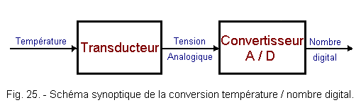
.gif)
 Click here for the next lesson or in the summary provided for this purpose.
 Top of page
 Next Page