All physical quantities (pressure, temperature, light intensity, speed, etc.) can be converted into electrical quantities (current, voltage) by means of specific components called transducers.
A microphone is an example of a transducer that converts a variation of ambient air pressure into an electrical voltage whose amplitude is a function of the pressure variation.
The microphone delivers an analog voltage, that is, a voltage that can take all possible values over a given interval.
An analog signal therefore has a minimum value and a maximum value.
A digital signal, on the other hand, takes only two logical values (1 and 0).
As a result, all digital circuits seen so far can not generate or process an analog signal.
To fulfill this function, it is necessary to insert at the input of the digital circuit, a device that converts the analog voltage or current into a digital signal : this device is called analog / digital converter.
Reverse conversion, that is to say from a digital signal to an analog signal, takes place through a digital-to-analog converter.
In the "digital electronic 14 theoretical lesson corresponding" to this practice, you have learned what are the characteristics of the converters and on what principles their operation is based.
In this practice, you will experiment these circuits and see some applications.
Remember that the main features of a digital to analog converter are :
Its resolution : it is the number of analog levels that we collect on its output.
This resolution is a function of the number of bits on which the converter operates.
The larger the number of bits, the higher the resolution. With 8 bits, the converter delivers 256 analog levels from 0 volt to the maximum voltage ; with 9 bits, there are 512 levels and so on.
Its accuracy : this parameter indicates the difference that can exist between the real voltage and the theoretical voltage. The accuracy is not related to the resolution a converter can have a low resolution, but a high accuracy.
Its linearity : a converter is linear if its output voltage is proportional to the binary number present on its input.
The end of scale (full scale) : it is the maximum value of the analog voltage that the converter can provide in output.
Its offset : is the value of the output voltage when all logic inputs are at zero. An ideal converter has zero offset voltage.
Prepare the following material to perform all the experiments that will follow :
1 integrated circuit ADC 0804
1 integrated circuit LM 335
1 integrated circuit LM 747
1 integrated circuit MM 74C00
1 integrated circuit MM 74C74
1 integrated circuit MM 74C154
1 integrated circuit MM 74C193
1 resistor of 2,7 kW
- 1 / 4 W - tolerance 5 %
1 resistor of 4,7 kW
- 1 / 4 W - tolerance 5 %
1 resistor of 5,6 kW
- 1 / 4 W - tolerance 5 %
3 resistors of 10 kW
- 1 / 4 W - tolerance 5 %
1 resistor of 22 kW
- 1 / 4 W - tolerance 5 %
1 resistor of 39 kW
- 1 / 4 W - tolerance 5 %
1 resistor of 82 kW
- 1 / 4 W - tolerance 5 %
1 resistor of 2,2 kW
- 1 / 4 W - tolerance 5 %
1 potentiometric trimmer of 1
kW
1 potentiometric trimmer of
10 kW
1 capacitor of 150 pF
2 capacitors of 0,1 µF
1 tantalum electrolytic capacitor of 10 µF - 10 Volts
1 braid of soft wire (red and black) of 0,25 mm².
2. - FIRST EXPERIENCE : EXAMINATION OF
AN OPERATIONAL AMPLIFIER
It is necessary to have some notions about the operational amplifiers, which are analog circuits, to approach the examination of the converters.
These are both analog components and digital components.
Operational amplifiers are general purpose integrated circuits from which an analog circuit can be designed.
The following experiment will allow you to check the operation and main characteristics of an operational amplifier.
In Figure 1 is shown the pinout of the integrated circuit LM 747 which will be used in the following experiments. This circuit comprises two independent operational amplifiers.
Each operational amplifier has an inverted input marked (-) and a non-inverting input denoted (+). If a signal is applied to the (-) input, the output signal is in phase opposition with respect to this input signal. On the other hand, if the signal is applied to the (+) input, the output signal is in phase with the input signal.
The operational amplifiers A and B of the LM 747 circuit can operate with a symmetrical power supply.
The positive power is applied to pins 13 and 9, while the common negative power is applied to pin 4.
In the following experiment, the negative power supply will be provided by a 4.5 volt battery.
Make sure that the battery is in good condition (new battery).
2. 1. - REALIZATION OF THE CIRCUIT
a) Remove from the matrix the links and components related to the previous experiment.
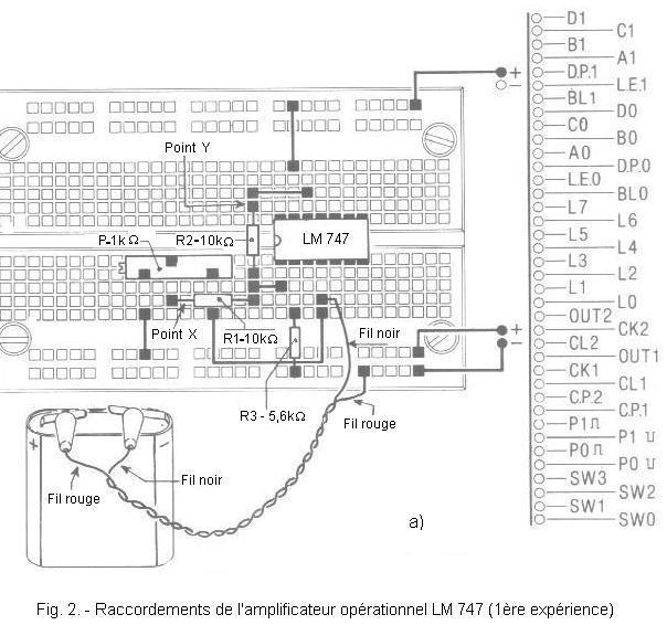
b) Insert the LM 747 integrated circuit on the matrix as shown in Figure 2-a.
c) Insert the other components and make the connections shown on this same Figure 2-a.
The Figure 2-b shows the electrical diagram of the assembly made.
Now you need to make a cord to connect the 4.5 volts battery to the matrix.
d) To do this, cut two pieces of soft wire, one red and the other black and solder two crocodile clips as shown in Figure 2-a.
At the other end of the two wires, solder a piece of tinned rigid wire about 1 cm long.
Insert the two red and black caps as shown in Figure 3 and twist the two wires together.
e) Connect the 4.5 volts battery using the cord as shown in Figure 2-a.
Note that this is the red wire that is connected to the mass of the digilab. Do not immediately connect the black crocodile clip to the (-) pole of the battery.
First try :
a) Connect the black crocodile clip to the (-) pole of the battery and turn on the digilab.
b) Prepare the controller for the measurement of voltage C.C. at 10 volts and measure the voltage Ve applied to the input of the amplifier. This voltage Ve is located between the point X which corresponds to a terminal of R1 and the mass of the digilab which is also the pole (+) of the battery.
This voltage can be positive, zero or negative depending on the position of the trimmer's cursor.
To measure Ve, place the black tip of the controller on the ground and the red tip on point X.
If the needle deviates to the left of scale 0, invert the two key points because Ve is negative.
c) Record the value of Ve in the left column of the table in Figure 4.
Fig. 4. - Table of the voltages Ve and Vs of the operational amplifier
Input voltage (Ve)
Output voltage (Vs)
d) In the same way measure the voltage Vs corresponding to Ve by connecting the test points of the controller to the point Y and to the ground.
e) Report this value in the second column (Vs) of the table in Figure 4. Each time, do not forget to indicate the sign of the measured voltage.
f) Carry out a series of measurements for Ve and Vs by playing on the trimmer P. You can thus browse all possible input values from - 4.5 volts to + 5 volts for example.
Put some values (Ve and Vs) in the table (Figure4).
Observe this table, you see that Ve and Vs are equal but of opposite sign, if you measure + 1.5 volts for Ve, Vs will be worth - 1.5 volts and so on.
g) We will calculate the G gain of the amplifier. We have the relationship :
For example, with Vs = - 1.5 volts and Ve = + 1.5 volts, gain = - 1.5 / + 1.5 = - 1
This circuit therefore has a unity gain (G = -1) and reverses the input signal.
You could also notice that there is a voltage range for the voltage Ve, for which the amplifier has a gain of -1, but beyond this range, this gain is no longer respected.
Indeed, the maximum output voltage is about + 4.5 volts and the minimum voltage at - 2.5 volts.
a) Remove the resistance R2 of 10 kW
(Figure 2),
connected between the pins 1 and 12 of the LM 747 and replace it by a resistance of 22 kW.
b) Connect the battery and turn on the digilab.
c) Carry out the same series of measurements as before and put all the values in a table identical to that of Figure 4.
This time you observe that, for a voltage Ve equal to + 1 volt, the output voltage Vs already reaches - 2.5 volts, that is to say the lower limit for the output of the operational amplifier. In the same way, when the voltage Ve reaches - 2 volts, the voltage Vs reaches the upper limit which is + 4.5 volts.
When the input voltage Ve is outside the range - 2 volts at + 1 volt, the amplifier is saturated.
The two limit values at the output of the amplifier are a function of the values of the positive and negative power supplies of the integrated circuit.
In general, an operational amplifier is supplied with voltages of values greater than those of the present experiment (for example + 15 volts and - 15 volts).
d) For this last test, the gain G is : G = Vs / Ve = - 2,2
This formula is only valid if the amplifier is unsaturated.
We obtain Vs = - 2.2 x Ve
e) Replace R2 with another 39 kΩ resistor and take a series of measurements as before. Be sure to stay in an input voltage range such that the amplifier is not in saturation.
Calculate the gain G
:
You have to find - 3,9 about.
Note :
Due to the tolerance on the values of the resistors R1 and R2 as well as the accuracy of the controller, the voltages noted during the tests, and consequently the calculated gains, can be significantly different from the values given in this practice.
For convenience, the value of the resistor R3 was not changed each time the value of R2 was changed. However, it would have been necessary to adapt for each series of measurements the value of R3.
We will come back to this problem.
These different tests allowed you to check the formula already seen in theory :
R2 is the feedback resistance and R1 is the input resistance.
In the first test, R1 = R2 = 10 kΩ and the gain G is - R2 / R1 = - 104 / 104 = - 1
In the second test G = - (2.2 x 10⁴) / 104 = - 2.2
For the last test G
= (3,9 x 10⁴) / 104 = - 3,9
In conclusion, we can give the following formula :
f) This experience is over, so turn off the digilab.
In summary, this experience has allowed you to see the operation of an operational amplifier mounted as an inverting voltage amplifier.
This operational amplifier requires two supply voltages, one positive, the other negative. This feature is common to many analog circuits.
Resistor R3, connected to the non-inverting input (pin 2) of the LM 747, has the function of minimizing the output offset voltage. This resistance R3 must be equivalent to the resistance that "sees" the inverting input.
The latter is constituted by the paralleling of R1 and R2 without omitting the trimmer in series with R1
The equivalent resistance of this trimmer for the inverting input varies from 0 Ω to 250 Ω. This resistance is zero when the trimmer's slider is located at one of the two ends and it is maximum (250 Ω) when the slider is located in the middle of the trimmer. In this case, we have 500 Ω in parallel with 500 Ω, which gives a value of 250 Ω.
Finally, we have (R1 + 250 Ω) in parallel with R2, that is 10 250 Ω // 10 kΩ which gives 5,061 Ω.


 Preparation of equipment
 Click here for the next lesson or in the summary provided for this purpose.
 Top of page
 Next Page