Realization of a Continuous Voltage Converter ... :
7. - FOURTH EXPERIMENT : REALIZATION OF A CONVERTER OF CONTINUOUS VOLTAGE
In some circuits, from a Continuous Voltage, it may be necessary to create a Continuous Voltage higher than the existing value. It may be useful to use a Continuous Voltage converter that can raise this voltage. For this, several types of circuits are possible. In this case, we will see a converter model using the LM 555 integrated circuit.
7. 1. - REALIZATION AND TESTING OF THE CIRCUIT
a) Remove from the matrix the connections and components related to the previous experiment, leaving in place only the LM 555 integrated circuit.
b) Perform the assembly shown in Figure 15.
The two test points of the controller are in contact with two pieces of stripped rigid wire and inserted into the matrix.
The electrical diagram of the realized circuit is located Figure 16.
c) Turn on the Digilab.
d) Prepare the controller
for the 10 V DC voltage measurement and put the contact tips in contact with the cathode of diode D1 (red tip) and with the ground (black tip) as shown in Figure 15.
You must find a voltage of about 8.8 volts.
e) Turn off the Digilab.
In conclusion, this circuit makes it possible to obtain a higher voltage than that supplying the circuit.
The integrated circuit LM 555 generates a rectangular signal whose frequency is :
This rectangular signal is applied to the input of a voltage doubler circuit consisting of two diodes and two capacitors as shown in Figure 17.
The operation of this voltage doubler is as follows :
When the input signal (rectangular signal) is at the level L, the diode D2 is forward biased and driven. Capacitor C3 charges and point A is at + 4.4 volts (Figure 18-a). On the other hand, D1 is reverse biased and no current flows through it.
Lorsque
When the input signal goes to the level H, the voltage variation thus created is transmitted through C3 and the point A is found at the potential + 9.4 volts (4.4 volts + 5 volts). Immediately the diode D2 stops driving (Figure 18-b), while D1 is forward biased and allows the capacitor C4 to charge. Point A being at + 9.4 volts the output will be at a potential of + 8.8 volts (we consider that the threshold of diodes D1 or D2 is 0.6 volt).
When the input signal returns to L level, the output remains at + 8.8 volts since C4 can not be discharged immediately.
You will find an output voltage of less than 8.8 volts (rather 8 to 8.5 volts) because the potential variation at the output of the multivibrator is always less than 5 volts.
It would be possible to obtain even higher output voltages. It would be enough for that to put several doublet of voltage in cascade.
With a doubler of voltage, we obtain 10 volts from 5 volts, with two doublers, we get 15 volts and so on.
If V is the initial voltage and N is the number of voltage doublers, the final voltage is : (N + 1) x V (volts).
The disadvantage of this experimental setup lies in the fact that the current available at the output is relatively low.
Nevertheless, there are converters based on this principle and capable of providing sufficient power to power an electronic circuit.
8 - FIFTH EXPERIENCE: REALIZING AN ANALOGUE
FREQUENCEMETER
In this experiment, the LM 555 is used for the design of a fairly simple frequency meter.
Although the accuracy of this one is rather weak, this circuit makes it possible to understand the principle of an analog frequencymeter.
8. 1. - REALIZATION OF THE CIRCUIT
a) While leaving the LM 555 circuit in place, remove the components and links related to the previous experiment.
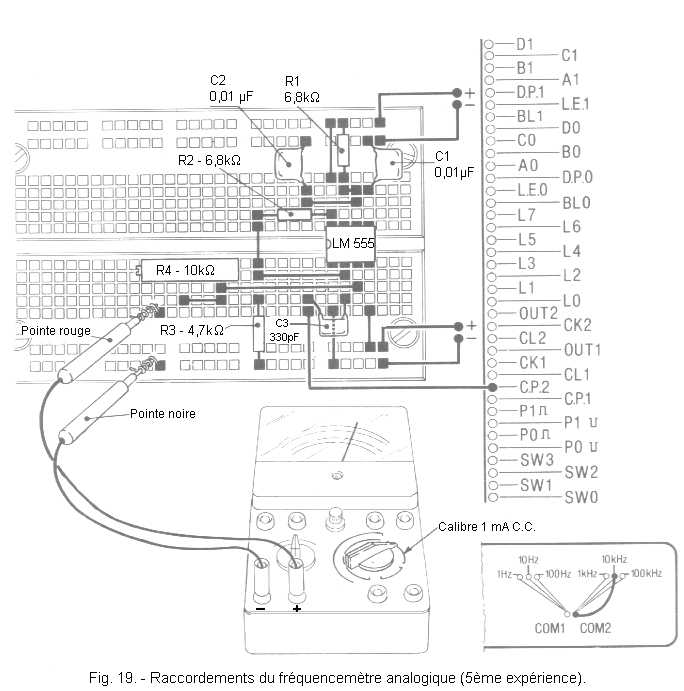
b) Insert on the matrix two capacitors of 0.01 µF, a capacitor of 330 pF, two resistors of 6.8 kΩ, a resistance of 4.7 kΩ and a trimmer of 10 kΩ in the positions illustrated in Figure 19.
c) Then perform the connections shown in this Figure 19.
The electrical diagram of the analog frequencymeter is given in Figure 20.
8. 2. - OPERATING TEST
a) Prepare the controller for 1 mA continuous current measurement and connect the negative (black) tip to the ground and the positive (red) tip to the free end of the 10 kΩ trimmer, as shown in Figure 19.
To connect the test probes, use two pieces of bare, rigid insulated wire that you wrap around the test probes.
b) Arrange the clock generator at 10 kHz.
c) Switch on the Digilab and turn the trimmer screw so that the galvanometer reads 1 mA (end of scale needle).
d) Set the clock generator to 1 kHz and read the value indicated by the galvanometer. It is about 0.1 mA.
e) Turn off the Digilab.
With the circuit you just realized, you get an analog indication of the value of a frequency. Indeed, the position of the galvanometer needle is directly a function of the frequency of the signal present at the input of the circuit. It would be enough to use an appropriate scale to read directly in Hz.
In this case, it is the 1 mA caliber which is used and the trimmer R4 serves as additional resistance so that the frequency of 10 kHz corresponds to the maximum deviation of the needle.
The indication of the galvanometer is proportional to the frequency. That is why at 1 kHz, the galvanometer indicates 0.1 mA.
At 5 kHz, it would indicate 0.5 mA, at 8 kHz it would also indicate 0.8 mA and so on.
The operating principle is based on measuring the average voltage of the monostable output signal.
The average value of the voltage of a periodic signal is calculated over a period.
In the case of the signal of Figure 21, the average value Vm is :
In the experiment circuit, for each transition of the clock signal from a level H to a level L, the monostable generates a pulse whose duration T is worth :
T = 1,1 R1 C2 =
1,1 x 6,8 x 103 x 0,01 x 10-6
T = 75 µS
At the output of the monostable, a rectangular signal is obtained whose frequency is identical to that of the tripping signal and each pulse lasts 75 µS.
Figure 22 represents the voltages Ve at the input of the monostable, Vt at the tripping input of the monostable and Vs at the output of the monostable in the two experienced cases.
The voltages Vt represent the differentiated input voltages Ve thanks to the network consisting of R2, R3 and C3 (Figure 20).
This makes it possible to have a very short trigger pulse with respect to the output pulse of the monostable. This problem was addressed during the digital theory 6 (pseudo-monostable). You notice that the monostable is triggered on the negative edge of the input signal.
At the rising edge of the input signal, a positive pulse is applied to the tripping input and then very quickly the voltage on the tripping input drops back to 2 volts (Vt = 2 volts).
Indeed, the ratio of resistors R2 and R3 imposes a potential of 2 volts on the tripping input.
Furthermore, let's not forget that the tripping comparator switches to 1.66 volt.
So when the input signal goes back to the L level, a negative pulse is created on the trigger input whose potential drops below 1.66 volt and the monostable triggers at that time.
If we look atFigure 22, we find that the ratio between the duration of the output pulse (75 µs) and the duration during which the output signal is at level L is directly proportional to the frequency of the input signal.
Indeed, when the frequency of the input signal is 10 kHz, the average value Vm1 of the output signal is :
Vm1 = VH x tH x F
= 5 x 75 x 10-6 x 10 x 103 = 3,75 volts.
In the second case, with F = 1 kHz, we obtain :
Vm2 = VH x tH x F
= 5 x 75 x 10-6 x 103 = 0,375 volt
It would therefore be possible to directly measure this average voltage with a galvanometer equipped with a voice coil because the latter can not follow rapid changes in voltage.
In the case that concerns us, we prefer to use the trimmer R4 and measure the current flowing through it, the latter being proportional to the average output voltage of the monostable.
This allows you to calibrate the galvanometer so that at 10 kHz the needle deviates to the maximum (1 mA).
The average current measured is Im = Vm / R ; R being the sum of the series resistors of the trimmer and the galvanometer.
It is a constant, so Im is well proportional to Vm and therefore to frequency.
Nevertheless, this measurement system is relatively imprecise, as much by the imprecision of the controller and the components as by the method by which the average value is obtained. To achieve more accurate measurements, more complex circuits with operational amplifiers would be required, but this would be beyond the scope of this course.
We will see how to perform this frequency measurement with a digital system.


 Realization of an Analog Frequency Meter
 Click here for the next lesson or in the summary provided for this purpose.
 Top of page
 Next Page